Snowflake Cost Calculator: Estimate Monthly Spend in Minutes
Use a snowflake cost calculator to estimate monthly spend in minutes. Learn formulas, worked scenarios, and optimization tips to avoid surprise bills.
You've got the familiar situation: the team has Snowflake running well enough to keep product moving, someone drops a few assumptions into the Snowflake cost calculator, and the number looks clean enough to share. Then the invoice lands and finance asks why reality is higher, messier, and harder to explain than the estimate. That gap is exactly where budgets drift, and it's where a calculator either helps or misleads.
The useful way to think about Snowflake is simple. The calculator is a planning tool, not a quote, and the bill is the result of compute, storage, and data transfer working together under workload patterns that rarely stay neat. Once you treat the calculator as the first pass in a broader FinOps workflow, it becomes a lot more valuable, because it forces the right questions before spend shows up.
Table of Contents
- Why Snowflake Bills Drift From the Estimate
- The Three Meters That Drive Every Snowflake Bill
- How Edition and Region Change the Calculator Output
- Walking Through the Official Pricing Calculator
- Two Worked Monthly Cost Scenarios
- The Five Inputs That Quietly Break Snowflake Cost Estimates
- From Calculator Estimate to Living Forecast
Why Snowflake Bills Drift From the Estimate
A data team I've seen more than once does the same thing on Monday morning. They estimate a tidy monthly figure, share it with leadership, and move on because the number feels directionally right. Then the bill arrives with a surprise attached, and the gap is big enough that finance wants a postmortem, not another spreadsheet.
The first reason the estimate slips is built into Snowflake's model. Compute is credit-based, and Snowflake notes that a credit is consumed only while compute resources are being used, with a 60-second minimum each time a warehouse starts or resumes. That minimum sounds small until workloads become bursty, because short jobs and repeated resumes pay for idle starts you didn't mentally budget for.
The second reason is storage creep. Active data isn't the whole story in Snowflake, because retention features like Time Travel and Fail-safe can keep historical data around and expand the storage line. The calculator can show storage assumptions, but it can't read your team's retention habits or the way those habits change after a quarter of convenience-driven defaults.
The third reason is transfer. Snowflake documents data transfer as a separate billed meter, and the rate depends on destination and region, which is exactly why same-region movement can look negligible while cross-region or internet egress becomes visible fast. Flexera's 2026 guide gives a concrete example of $0.00 per TB for same-region AWS US East transfer and $90.00 per TB for different-provider or internet transfer in that region, so a calculator that ignores transfer type is missing a real bill driver. For a broader cloud-cost management angle, this practical cloud cost article maps well to the same discipline.
Practical rule: if the calculator output looks comforting without naming warehouse cadence, storage retention, and transfer paths, it's probably undercounting something.
The right conclusion isn't to distrust the tool. It's to use it as a forcing function, then validate the estimate against actual consumption once the workload starts behaving like a real workload, not a lab demo.
The Three Meters That Drive Every Snowflake Bill
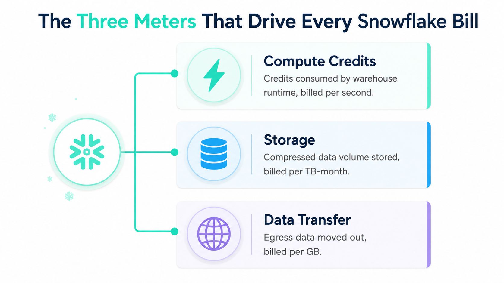
A Snowflake bill becomes easier to read once you split it into three meters. The calculator is only useful when you can map each input to a real charge, because then the estimate is a working model instead of a number on a screen.
Compute credits
Compute is usually the first line teams model, and for good reason. Snowflake says compute resources consume credits, and currency reporting converts those credits using the daily price of a credit. The practical formula is simple.
Compute cost = credits consumed × credit price
Snowflake's documentation shows one usage example where 4,464 credits at $2 per credit = $8,928. That is enough to show why warehouse size and runtime usually drive the biggest swings in the bill, especially when small jobs start and stop often. The same pattern shows up in other warehouses too, including the cost structure described in this Snowflake vs. Redshift cost comparison, where compute behavior still dominates the estimate.
Storage
Storage is easier to miss because it grows without much notice. The formula is straightforward.
Storage cost = compressed TB stored × monthly storage rate
In the same documented example, Snowflake shows 65 TB at $23 per TB = $1,495. Combined with compute in that example, that produces a billed total of $10,423, which is a useful anchor because it shows storage sitting beside the warehouse line instead of hiding under it. See Snowflake's worked breakdown in its overall cost explanation.
Data transfer
Transfer is the meter that surprises teams when data moves between regions, clouds, or the internet. The practical model is clear.
Transfer cost = data moved × applicable transfer rate
Flexera's guide shows same-region AWS US East transfer at $0.00 per TB and different-provider or internet transfer at $90.00 per TB in that region. That spread is why the calculator has to know where data is going, not just how much compute ran.
A useful calculator output is one you can explain line by line with this three-meter model. If you cannot do that, the estimate is probably missing a cost driver that finance will notice later.
How Edition and Region Change the Calculator Output
The two dropdowns many users rush past are the two that most often change the answer. Edition and region don't just decorate the estimate, they can move the bill enough to break a budget conversation if you leave them vague.
| Snowflake Edition Comparison for Cost Planning | ||
|---|---|---|
| Edition | Approx. credit price in US AWS | Key cost-relevant features |
| Standard | About $2 per credit in US AWS regions | Core warehouse usage, baseline planning |
| Enterprise | Higher than Standard | Multi-cluster warehouses and broader operational features |
| Business Critical | Higher than Enterprise | Database failover, HIPAA support, customer-managed keys |
The pricing guides in 2026 are consistent on the main point, even when exact contracts differ. The default on-demand rate in US AWS regions is about $2 per credit for Standard edition, while other editions and non-U.S. regions price differently. That means the same warehouse pattern can look cheap in one environment and meaningfully more expensive in another.
What the edition choice really changes
Standard is fine for teams that want baseline warehouse functionality and a clean forecast. Enterprise is where many teams start paying for operational flexibility, especially when concurrency and resilience matter. Business Critical is the tier that usually comes up when governance, failover, or regulated workloads enter the discussion.
Why region matters just as much
Region can be the hidden multiplier because cloud provider and geography shape both compute and transfer assumptions. Snowflake's own calculator asks for cloud provider and region first for a reason, and the result changes if you're on AWS, Azure, or GCP. That's also why a “Snowflake monthly cost” estimate without a named region is mostly a placeholder.
Budgeting rule: if someone says, “Snowflake costs about X,” the next question should always be, “On which edition and in which region?”
For teams comparing cloud economics, this Azure savings plans reference is a useful reminder that the cloud bill is always shaped by placement, not just raw usage. Snowflake behaves the same way, only with credit math instead of instance math.
Walking Through the Official Pricing Calculator
Snowflake's official Pricing Calculator is a free estimation tool, and that matters because you can use it early without asking procurement for permission. Snowflake's own FAQs say it provides estimated costs only, and results vary by region, workload, and other variables, so the correct expectation is a planning estimate, not a final invoice.
Start with cloud provider and region. Those two fields set the environment for the rest of the estimate, and they're the first place teams accidentally generalize from one deployment to another. Then choose the edition, because the calculator needs to know whether you're modeling Standard, Enterprise, or Business Critical behavior.
Put workload shape into the compute fields
The next input is usually warehouse sizing and usage time. A mid-size SaaS workload often looks more like a couple of steady BI and engineering warehouses than one giant warehouse that runs all day, so a reasonable example is two Medium warehouses running 6 hours a day. That kind of pattern gives the calculator something meaningful to work with, because it captures both concurrency and runtime instead of pretending the platform behaves like a single monolithic job.
Add storage and the extras most teams forget
Enter storage in compressed TB, not raw source-system size. Then account for AI features, add-ons, and any optional services your environment uses, because Snowflake's calculator is designed to estimate more than just warehouse runtime. If you're only typing a warehouse number and ignoring everything else, you're leaving the biggest surprise charges out of the estimate by default.
A clean workflow is to think in workload classes, not line items. BI, ingestion, data science, and AI can each have different runtime patterns, different storage growth, and different transfer behavior, so folding them into one average can make the result look precise while being wrong.
Good practice: use the calculator to pressure-test the assumptions, then immediately compare those assumptions with usage views once the workload is real.
The calculator can still save time and money because it shortens the path to a defensible first budget. It just shouldn't be treated as the last word on cost.
Two Worked Monthly Cost Scenarios
A calculator gets real when you can walk the math yourself. These examples don't require magical inputs, just the same three meters used consistently, which is why they're useful for sanity-checking whatever the Snowflake interface spits back.
BI-heavy team on one warehouse
Take a team that runs a single Small warehouse for 4 hours a day, keeps 5 TB of compressed storage, and sends only minimal data out. The compute side is the only part that really moves here, so the month starts with warehouse runtime and then adds storage.
If the warehouse behaves predictably, compute is credits consumed over the month multiplied by the applicable credit price. Storage is 5 TB times the storage rate, and transfer is close to negligible if the team keeps most traffic in the same region and cloud. This is the sort of workload where a calculator is helpful, because the estimate usually matches the mental model reasonably well.
Data engineering team with cross-region movement
Now flip to a heavier pipeline team running two Large warehouses, auto-suspend tuned for streaming jobs, 40 TB of storage, and cross-region movement. The compute estimate climbs because both warehouse size and concurrency are higher, storage becomes material because the retained footprint is larger, and transfer stops being a rounding error when data leaves the region.
The point of this contrast is not to force a precise dollar total from thin air. The point is to show how a monthly number should be built, line by line, so the team can tell whether an estimate is plausible before finance ever sees it.
Sanity-check against Snowflake's own example
Snowflake's documented example is a useful anchor for this kind of review. It shows 4,464 credits at $2 per credit = $8,928 for compute, 65 TB at $23 per TB = $1,495 for storage, and a $10,423 total billed cost in that scenario. If your own modeled number looks wildly different from the workload shape you described, the estimate probably needs another pass.
A useful habit is to write the arithmetic beside the assumptions before anyone shares the number upward. That simple step saves time later because finance can see which line item moved instead of asking you to reconstruct the whole estimate from memory.
The Five Inputs That Quietly Break Snowflake Cost Estimates
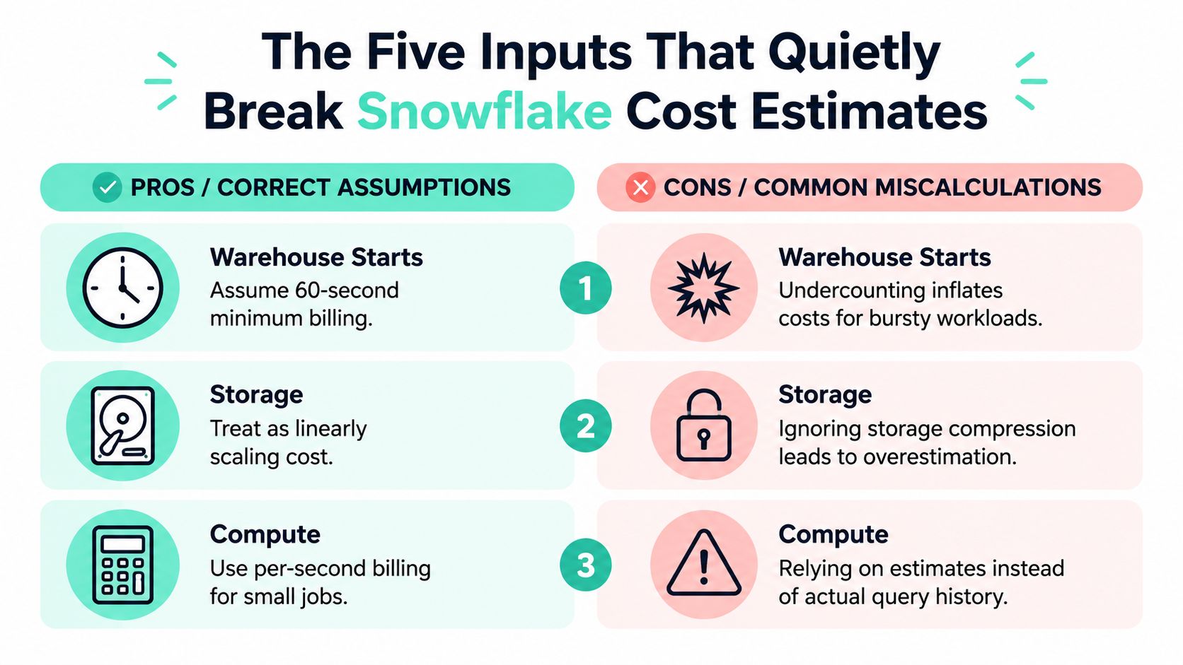
The worst calculator errors usually come from inputs that feel “close enough.” They aren't. They're the places where a small modeling mistake becomes a finance conversation later.
- Warehouse starts: A bursty workload with repeated resumes pays the 60-second minimum every time the warehouse starts or resumes, so a few short jobs can cost more than an hourly average suggests.
- Storage sizing: Treat compressed TB as the input, not raw source data, or the estimate becomes distorted before it ever reaches the bill.
- Retention settings: Time Travel and Fail-safe can keep historical data around, which means storage assumptions that ignore them are usually too low.
- Transfer path: Same-region movement can be very different from cross-region or internet egress, and Flexera's example shows how wide that gap can be in practice.
- Workload shape: A single warehouse-hours figure can hide concurrency, multi-cluster behavior, and mixed workloads, which makes the estimate look cleaner than it is.
A simple example makes the problem obvious. If a team assumes one long-running warehouse and then shifts to short, repeated resumes, the 60-second minimum makes the cost rise even if query duration looks stable. If the same team also moves analytics exports across regions, the transfer line can become visible fast.
The calculator won't ask those follow-up questions for you. It assumes you'll know where the shape of the workload differs from the shape of the form.
One more practical point. Teams often blame the calculator when the mistake was in the inputs, especially around storage compression and transfer destination. That's not a tool failure, it's a modeling failure.
Rule of thumb: if the estimate depends on a single average warehouse-hours number, it's probably too coarse for anything beyond a first budget draft.
For teams that want a broader cost-allocation workflow, this guide on cost allocation methods fits neatly beside Snowflake cost review. The same discipline applies, name the driver, then measure it as close to the source as possible.
From Calculator Estimate to Living Forecast
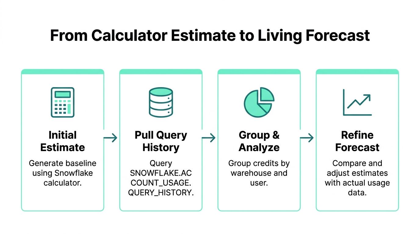
The calculator gives finance a starting number. Discipline comes from making that number survive contact with usage data, which is why Snowflake's own usage views matter as much as the original estimate.
Reconcile estimate to actual usage
A strong reconciliation workflow starts with SNOWFLAKE.ACCOUNT_USAGE.QUERY_HISTORY, then groups queries by warehouse and cluster, allocates interval credits proportionally to active share, and rolls the results up by query text when a team needs attribution detail. A simpler option uses warehouse_metering_history and allocates credits by execution-time share, which is often enough when the goal is monthly planning rather than per-query chargeback.
Snowflake doesn't expose exact per-query credit contribution, so any allocation rule is still an approximation. That's the critical truth most calculator guides skip, and it matters because the finance team needs a method that is repeatable even when it isn't perfectly exact.
Use the views as a monthly habit
Snowflake's own documentation points users to Snowsight and the ACCOUNT_USAGE and ORGANIZATION_USAGE views for historical consumption review, which makes those views the reconciliation layer between estimate and invoice. That's where the calculator stops being a one-time artifact and becomes part of a monthly process. Teams that keep this habit usually spot variance earlier, before the invoice becomes a surprise.
The practical playbook is straightforward. Tighten auto-suspend so idle warehouses don't drift, right-size warehouses to actual query concurrency, prune Time Travel retention where the business doesn't need it, and prefer same-region transfer paths whenever possible. Then add a 20 to 30% variance buffer to the initial estimate and revisit the model every quarter so finance isn't planning around stale assumptions.
What actually works in practice
The teams that stay ahead of Snowflake spend don't chase perfect estimates. They keep the calculator, the usage views, and the monthly budget conversation tied together so the estimate gets sharper over time instead of older.
If you want tooling for that broader pattern, SpendLens AI is one option for attributing and reviewing usage-based AI spend in a similar workflow, especially when teams need clear drivers and recurring reporting across workloads. The same logic applies to Snowflake, estimate first, then reconcile the consumption path against the model.
The calculator is the right place to start a Snowflake budget conversation, but it's the ACCOUNT_USAGE views that keep it honest.
If you want a tighter cost workflow around recurring usage bills, visit SpendLens AI and compare how it structures spend attribution, reporting, and savings opportunities. It's a practical next step for teams that want the same kind of control over usage-based costs that Snowflake teams need from the calculator and the usage views.