
AI Infrastructure Cost: What Really Drives the Bill
AI infrastructure cost breaks down into compute, inference, data, storage, and networking. Learn what drives spend and how to forecast and control it.
The popular advice is to “buy the right GPUs” and treat the purchase as the AI budget. That advice misses the bill many struggle to control. AI infrastructure cost is becoming a recurring inference and attribution problem, shaped by token volume, model selection, prompt length, cache behavior, utilization, networking, and the supporting power and cooling stack.
The scale of the physical infrastructure makes that clear. Global data center capital expenditure rose 51% to $455 billion in 2024, with accelerated servers optimized for AI workloads attributed as the main growth driver, according to Dell'Oro's data center CapEx analysis. Yet a production team can still lose control of spend without owning a hyperscale facility. A shared API key, an oversized prompt, or an agent retry loop can hide the responsible product behind one aggregate invoice.
The practical question isn't how much compute AI needs. It's which workload generated the cost, which unit economics explain it, and which change can lower the next monthly variance report.
Table of Contents
- Why AI Infrastructure Cost Is Really an Inference Problem
- The Main Cost Components of AI Infrastructure
- How Model Pricing and Caching Change the Equation
- Why the Same Token Count Can Produce a Very Different Bill
- Attribution Challenges That Make AI Bills Hard to Forecast
- High-Level Strategies to Control and Forecast AI Spend
- A Practical Plan to Reduce and Forecast AI Infrastructure Cost
Why AI Infrastructure Cost Is Really an Inference Problem
The GPU purchase narrative is attractive because hardware is visible. A procurement request has a price, a capacity plan, and an amortization schedule. Inference is less tidy. It creates a recurring run rate that grows with user activity, prompt size, generated output, retries, and the percentage of traffic routed to expensive models.
That distinction matters even more as organizations move from experiments to production. Gartner's August 2026 forecast places AI-optimized infrastructure spending at $42.3 billion in 2026, with inference at $23.3 billion, ahead of training at $19 billion. The same forecast projects inference at 59% of AI-optimized infrastructure spending in 2027. These figures make the budgeting shift explicit. Training may be a major project expense, but inference becomes an operating obligation after launch. (TechSignal's summary of the Gartner forecast)
A useful primer on the serving side is what LLM inference means in production. The key FinOps implication is that the invoice follows activity, not depreciation. A self-hosted GPU pool incurs cost through allocated GPU-hours, while a managed API exposes the same pressure through input and output tokens.
Practical rule: Treat every production inference request as a billable business event, not merely an application log entry.
The cost categories behind the run rate
The recurring bill usually combines:
- Compute: GPU-hours, utilization, memory capacity, and capacity held for latency objectives.
- Inference: Input tokens, output tokens, cache reads and writes, model tiers, and retries.
- Data: Ingestion, embedding generation, retrieval, and vector database operations.
- Storage: Datasets, model artifacts, checkpoints, logs, and archives.
- Networking: Egress, cross-region traffic, replication, and private connectivity.
- Vendor mechanics: Pricing tiers, context rules, batch options, and caching policies.
The attribution problem cuts across all of them. API providers may show usage under a small number of accounts or keys, while an application routes traffic from multiple teams, tenants, features, and environments. Without request-level metadata, finance can see that spend increased, but not whether a new feature, a customer cohort, a prompt release, or a retry regression caused it.
The solution isn't to predict one perfect monthly number. It's to establish unit economics that engineering can influence this month, such as cost per completed task, cost per 1,000 tokens by workload, cache-hit rate, GPU utilization, and cost per tenant. Those measures turn an opaque bill into an operating system for decisions.
The Main Cost Components of AI Infrastructure
A 1-gigawatt AI data center provides a useful magnitude anchor because it exposes how far the economics extend beyond model calls. One analysis estimates $38 billion in upfront CapEx, $0.9 billion in annual OpEx, and roughly $8.5 billion in annualized total cost of ownership for such a facility. Servers represent about $5.0 billion per year, or 60% of annualized cost, while facilities account for about $1.4 billion and networking about $1.2 billion. (Epoch AI's AI data center cost breakdown)
The exact scale differs for a SaaS team using APIs, but the structure remains useful. Each layer has a cost unit and a metric that can reveal variance before the invoice arrives.
Compute is more than the GPU hourly rate
Servers dominate the 1GW annualized cost profile. That includes accelerators, memory, interconnect pressure, and the capacity needed to meet throughput and latency requirements. A GPU that spends much of its time waiting for requests can still generate a full capacity charge, so realized work per GPU-hour is more informative than allocated capacity alone.
For self-hosted systems, track GPU utilization alongside tokens per second, queue time, and cost per successful request. For shared pools, allocate GPU-hours by job, namespace, model, or tenant. The optimization lever is usually utilization before procurement. Improving batching or moving suitable traffic to a smaller model can defer additional hardware.
Inference creates the recurring operating bill
Inference cost includes both managed API usage and self-hosted serving. During decode, each generated token requires repeated reads of model weights and KV-cache data, which can make production serving memory-bandwidth-bound rather than raw-compute-bound. The resulting cost per token depends heavily on realized tokens per second and the GPU hourly rate. (Technical analysis of memory bandwidth in LLM inference)
Measure cost per 1,000 input tokens, cost per 1,000 output tokens, tokens per second, cache-hit rate, and cost per completed workflow. Load, latency SLOs, and autoscaling policy belong in the same dashboard because idle standby capacity is part of the serving decision.
Data, storage, and networking hide outside the model invoice
Data costs appear through ingestion pipelines, embedding generation, retrieval, and vector databases. The right metric is cost per indexed document, retrieval cost per request, or cost per successful retrieval, depending on the architecture.
Storage accumulates through training datasets, checkpoints, model artifacts, logs, and cold archives. Track $/GB-month by lifecycle class and separate hot operational data from material that can move to colder storage.
Networking becomes visible through $/TB egress, cross-region replication, private interconnect, and movement between services. A retrieval architecture can look efficient at the model layer while creating unnecessary data transfer through poor regional placement.
| Cost Component | Share of 1GW Spend | Primary Cost Unit | Key FinOps Metric |
|---|---|---|---|
| Servers and compute | $5.0 billion per year, 60% of annualized cost | GPU capacity and throughput | Cost per GPU-hour, tokens per GPU-hour |
| Facilities | $1.4 billion per year | Power, cooling, site, and operations | Cost per deployed MW |
| Networking | $1.2 billion per year | Fabric and data movement | $/TB egress, cost per request |
| Inference workload | Included within server and operating layers | Input and output tokens | Cost per 1,000 tokens |
| Data and storage | Not separately quantified in the 1GW breakdown | Ingestion, retrieval, and GB-month | Cost per document, $/GB-month |
The conclusion is operational: compute is the largest physical layer, but inference, data, storage, and networking determine whether each unit of that capacity produces useful work.
How Model Pricing and Caching Change the Equation
Token counts don't have one universal value. Providers price input and output separately, and generated output is often the more expensive side of the transaction. The precise rate depends on model and tier, so a routing policy that treats every request alike can turn a manageable workload into an avoidable run-rate problem.
OpenAI's pricing page gives concrete examples. One tier lists $4.00 per 1 million input tokens, $0.40 per 1 million cached input tokens, and $20.00 per 1 million output tokens. A lower tier lists $0.20 input, $0.02 cached input, and $1.20 output per 1 million tokens. (OpenAI API pricing) Anthropic's documented caching model uses cache reads at 0.1x the base input price, with cache writes priced at 1.25x for a 5-minute cache and 2x for a 1-hour cache. One Sonnet-class example lists $3.75 per 1 million tokens for a 5-minute cache write and $0.30 for a cache read. (Anthropic pricing guidance)
Compare the unit economics before comparing vendors
| Model | Input $/1M | Cached Input $/1M | Output $/1M | Context Premium |
|---|---|---|---|---|
| OpenAI example tier | $4.00 | $0.40 | $20.00 | Depends on tier and context rules |
| OpenAI lower tier | $0.20 | $0.02 | $1.20 | Depends on tier and context rules |
| Anthropic Sonnet-class example | Base price varies | $0.30 in the cited cache path | Model-dependent | Cache duration changes write economics |
| GPT-5.5 comparison listing | $5.00 | $0.50 | $30.00 | Context and tier rules matter |
| Anthropic Claude Opus comparison tier | Flat across its full context window | Provider rules apply | Model-dependent | Full-window pricing can differ materially |
The comparison should focus on effective cost for the actual request shape, not the headline input rate. Long contexts can carry different pricing mechanics, and a model's full context policy can change the result even when two base prices appear similar. Independent comparisons list GPT-5.5 at $5 input, $30 output, and $0.50 cached input per 1 million tokens, while describing a Claude Opus tier with flat pricing across its full context window. (OpenAI and Anthropic pricing comparison)
Caching turns repetition into a design variable
Caching works best when a request repeats a stable system prompt, policy block, tool definition, or reference context. The first request pays the write treatment, but later reads can be dramatically cheaper. The break-even point depends on the write surcharge and the number of repeated reads, so teams should measure cache hits rather than assume that caching is active.
For example, a workload with a large reusable instruction prefix should compare uncached input cost against the write charge plus repeated read charges. A request router can then send stable, high-volume traffic to a cache-compatible path while keeping unique, short prompts on a simpler route. The resulting savings aren't universal, but cacheable workloads can reduce effective token cost substantially when the system records hit rate and verifies output quality.
Use an LLM pricing comparison to structure the evaluation, then validate current provider rates before changing production routing.
Why the Same Token Count Can Produce a Very Different Bill
Two production workflows process the same daily token volume. One is a retrieval-heavy chatbot with a large reusable context prefix. The other is an agent that repeatedly calls tools, resends its system prompt, generates extra reasoning, and retries failed actions. The token counter may show parity at the top level, while the invoice reflects four different economic realities.
Consider Workload A, a retrieval-heavy RAG chatbot using GPT-4o with large cached context prefixes. Much of its input is reusable, so cache reads lower the effective input rate. Its response path is direct, and the application limits retries when retrieval returns an incomplete result.
Workload B uses Claude 3.5 Sonnet for an agentic tool-calling workflow. It resends full system prompts, generates frequent reasoning tokens, calls tools several times, and re-queries after tool failures. Even with the same one-million-token daily total, the second workload can cost 4x more if its model tier, cache-hit rate, reasoning overhead, and failure behavior combine unfavorably. That is a scenario illustrating the economics, not a measured case study.
Four variables break token-count parity
- Model selection: A large model can carry a higher input and output rate, while a smaller model may handle classification, extraction, or deterministic routing.
- Caching state: The same prompt costs differently when a prefix is a cache write, a cache read, or an ordinary uncached request.
- Reasoning and tool use: Internal steps and tool responses can expand the billed workload beyond what the user sees.
- Failure-driven re-queries: Retries multiply both model calls and the context resent with each call.
The practical fix is to create a cost profile by workflow, not just by provider. Record model, input tokens, output tokens, cache status, tool-call count, retry count, and completed outcome. Then test whether enabling caching, reducing reasoning effort on deterministic steps, or enforcing a retry budget lowers cost per successful task without degrading the task's acceptance rate.
Attribution Challenges That Make AI Bills Hard to Forecast
Traditional FinOps systems begin with cloud accounts, services, instances, and environments. LLM spend often arrives as an aggregate from a few vendor accounts, leaving the bill unable to identify the product feature, team, tenant, or workflow behind each call.
The allocation problem becomes sharper when shared assets serve different workloads. One prompt template may support customer service, internal search, and evaluation jobs. Shared embeddings and vector indexes blur ownership, while batch jobs can fan out across teams under a single process name. Token totals alone therefore provide weak forecasting inputs because they hide the workload mix, ownership, and release changes behind demand.
A 2025 state-of-AI-cost-management report found that 85% of companies miss AI cost forecasts by at least 10%, while data platforms were the top source of unexpected AI spend at 56%. (PR Newswire's report summary) The implication for FinOps is direct: teams need an allocation layer that converts vendor charges into forecastable workload units before they can size optimization opportunities.
Build the allocation layer at the request boundary
Start with stable workload identifiers in API gateway headers, metadata fields, or application instrumentation. Each inference record should carry team, product, environment, feature, tenant, model, and release fields. Propagate those identifiers to retrieval calls, embedding jobs, and agent sessions where the architecture permits. A consistent schema also supports AI cost allocation methods across shared services.
Use the resulting data to compare model choice with task requirements. A routing service can find requests sent to a frontier model even though a smaller model may meet the acceptance criteria. The review should pair projected cost changes with evaluation results and migration risk, so a lower rate does not become a quality regression.
Prompt-waste detection adds a separate control. Flag oversized system prompts, repeated instructions, duplicated context, unbounded retrieval results, and unusually long outputs. Track each signal against input tokens per completed task, cache eligibility, and task success. That connects an engineering change to a measurable forecast variable.
Allocation also needs an operating owner. Finance can define reporting dimensions, platform teams can enforce metadata at the gateway, and application teams can validate feature and tenant labels. Begin with the highest-spend workflows, estimate avoidable tokens or plausible model downgrades, and record the expected monthly dollar effect before funding a tagging or routing project.
High-Level Strategies to Control and Forecast AI Spend
Teams often pursue too many optimizations at once. A better approach is to rank the levers by implementation effort, forecast value, and risk to output quality. The right first move depends on whether the current problem is model overuse, repeated context, poor utilization, uncontrolled tenants, or an absence of measurement.
| Strategy | Implementation Effort | Typical Savings | Forecasting Impact | Quality Risk |
|---|---|---|---|---|
| Right-size models by query class | Moderate | Workload-dependent | High, because model mix becomes explicit | Medium, requires evaluation |
| Prompt and response caching | Low to moderate | High on repeated context | High, cache-hit rate becomes forecastable | Low if cache invalidation is correct |
| Request batching | Moderate | Workload-dependent | Medium, separates asynchronous demand | Low for non-real-time work |
| Intelligent model routing | Moderate to high | Workload-dependent | High, connects request class to price tier | Medium if routing tests are weak |
| Tenant rate limits | Low to moderate | Prevents uncontrolled growth | High, creates bounded demand | Medium if limits affect service |
| AI FinOps tooling | Moderate | Enables targeted savings | High, improves attribution and variance analysis | Low, unless instrumentation adds latency |
Right-sizing is usually the cleanest architectural lever. Define query classes such as extraction, classification, summarization, retrieval response, and complex reasoning. Test a lower-cost model on representative samples, then promote it only when quality and business acceptance remain within the required threshold.
Caching deserves priority when prompts contain stable policies, tool definitions, or reference material. Measure cache-hit rate and uncached duplicate content. A cache policy that looks attractive on paper can underperform if small prompt changes constantly invalidate the prefix.
Batching is suited to evaluations, document processing, and other work that doesn't need interactive latency. Routing should combine model choice with workload urgency. A deterministic classification request shouldn't consume the same tier as an open-ended reasoning task.
Rate limits protect the forecast from tenant behavior and runaway agents. Set limits by product, tenant, or session, then connect them to alerts and an approved exception process. This is a governance control, not merely a traffic control.
Dedicated AI FinOps tooling becomes valuable when provider dashboards can't reconcile spend to workloads. Instrumentation should feed the monthly variance report with model mix, token mix, cache efficiency, retry volume, and cost per outcome. Savings only count when they remain visible after the next deployment.
A Practical Plan to Reduce and Forecast AI Infrastructure Cost
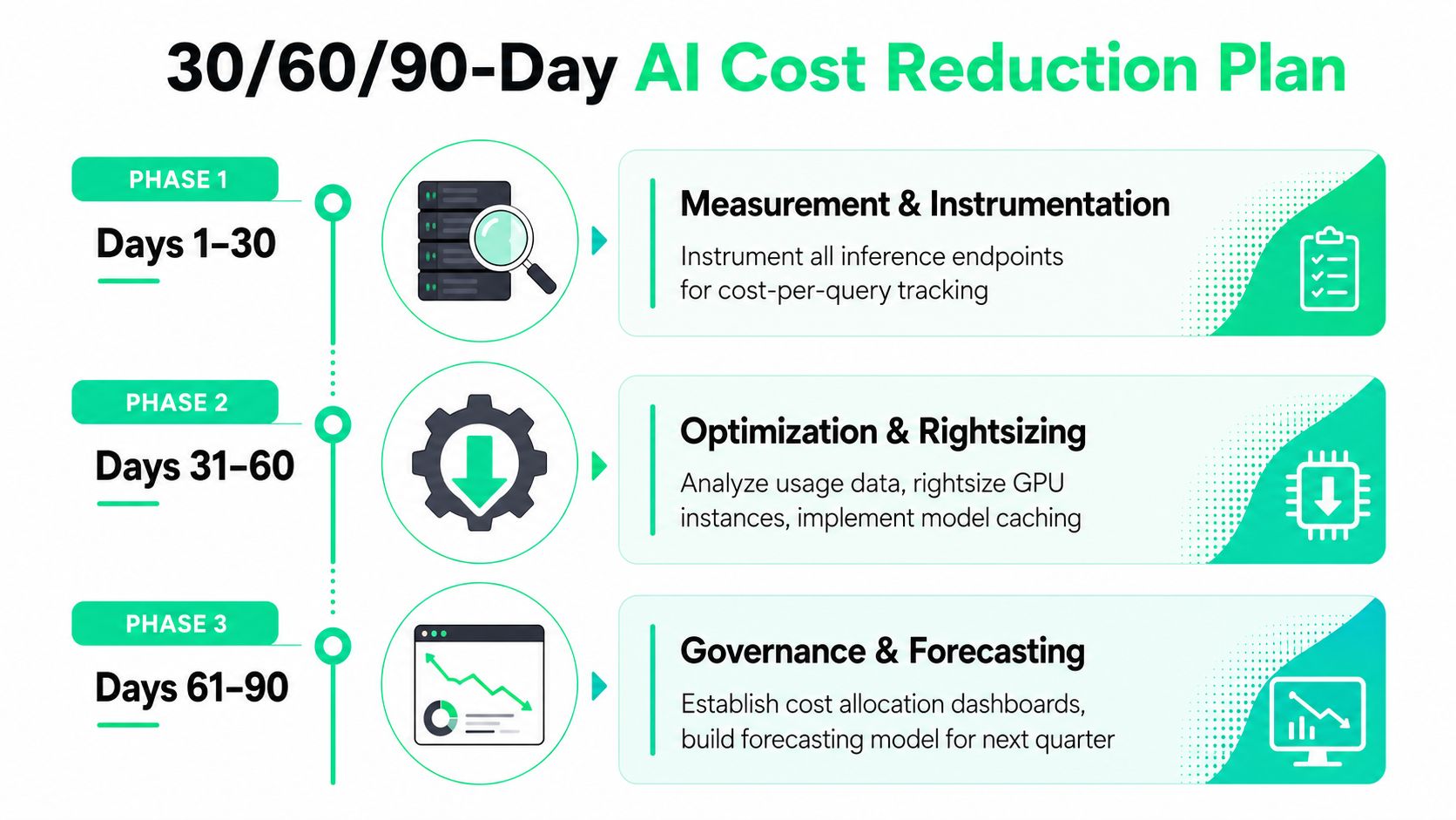
A 30/60/90-day plan works because it sequences visibility before optimization and optimization before commitment. Engineering can execute the first steps with existing services, while finance gains a defensible baseline for the next planning cycle.
Days 1 to 30, measure before changing traffic
The owner is the platform or FinOps lead, with application teams responsible for adding metadata. Instrument every inference call with model, input tokens, output tokens, cache-hit status, tenant, feature, environment, and release identifiers. Reconcile internal telemetry with vendor invoices and produce a workload-level leakage report.
The deliverable is a daily dashboard showing cost per request, cost per 1,000 tokens, cost per completed outcome, model mix, cache efficiency, and retry volume. The target metric is complete attribution for production inference, not an assumed savings percentage.
Days 31 to 60, capture low-risk savings
The engineering owner should enable prompt caching for stable prefixes, route simple queries to smaller models, batch non-urgent traffic, and set per-tenant rate limits tied to budget alerts. Each change needs a before-and-after comparison using the same quality measure, such as task acceptance, escalation rate, or retrieval success.
Set a target such as cutting blended cost per 1,000 tokens by 25%, but treat it as an internal objective rather than a guaranteed industry outcome. The deliverable is a change log that records the affected workflow, traffic share, measured cost movement, quality result, and rollback condition.
A saving without attribution is only a lower invoice. A saving with attribution becomes a repeatable control.
Days 61 to 90, turn usage into a forecast
Finance and engineering should build a rolling 90-day model using workload volume, seasonality, model mix, cache behavior, and planned feature launches. The monthly review should include engineering, product, and finance, with owners assigned to every material variance.
The target is to tighten forecast variance to within 10%, matching the explicit planning objective rather than claiming that every team will achieve it. The deliverable is a forecast with scenario inputs for adoption, model routing, prompt changes, and agent behavior.
For a structured estimation workflow, use AI cost estimation guidance. A platform such as SpendLens AI can add lightweight instrumentation, break down spend by project, provider, model, and workload, surface cache efficiency and prompt-waste signals, and recommend lower-cost model alternatives with estimated savings and migration risk.
The video below provides a visual companion to the operating model.
The immediate value is time saved during monthly close and incident review, because engineers no longer need to reconstruct ownership from raw provider exports. The financial value comes from making each optimization test measurable, attributable, and visible in the next forecast.
SpendLens AI helps teams instrument OpenAI and Anthropic calls, attribute spend by workflow and feature, expose cache efficiency and prompt waste, and identify lower-cost model-switch opportunities. Visit SpendLens AI to connect AI usage telemetry to the cost drivers and forecasts your engineering and finance teams need.