What Is LLM Inference: A Practical Guide for 2026
Learn what is LLM inference, how prefill and decode work, and why token shape drives AI spend. Practical guide for engineering and FinOps teams.

LLM inference is where the budget gets real. Training grabs attention, but inference is the line item that keeps growing every time a product ships a new prompt, a longer context, or another user-facing workflow.
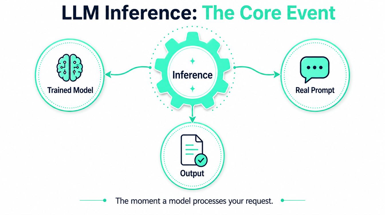
The useful way to think about what is LLM inference is simple, it's the moment a trained model processes a real prompt and returns a real output, and that single event is what gets billed, slowed down, cached, throttled, or broken in production. In practice, one call is a trained model plus a prompt plus serving software plus hardware, all turning into a response your app can show or store.
Table of Contents
- A Working Definition of LLM Inference
- The Inference Loop Step by Step
- Prefill and Decode as Two Different Cost Regimes
- Inference Types and Where Each One Fits
- The Cost Model Behind Every Inference Call
- Failure Modes You Will See in Production
- An Optimization Playbook for Engineering and FinOps
- Choosing Between Optimize Serving and Switch Models
A Working Definition of LLM Inference
The core idea behind what is LLM inference is straightforward. A trained model receives a real prompt and returns a real output. That output can be an answer, a summary, a classification, or a tool call that feeds another system. For a practical example of how teams expose that behavior through an API, see the OpenAI Completions API guide.
Inference is also the point where a model stops being an asset on paper and becomes a billable production service. The training run may be finished, but every prompt you send now consumes compute, memory, and serving capacity. In practice, that is where latency and spend start to matter.
A useful mental model is model plus prompt plus hardware plus serving stack equals one inference call. The model supplies capability, the prompt supplies work, the hardware supplies throughput, and the serving layer decides whether the call is cheap, fast, or both.
A customer-support summarization feature makes this concrete. A user closes a ticket, the system sends the conversation history to the model, and the model returns a short summary that gets stored in the CRM. That looks like a small product feature, but every extra reply, repeated instruction, or bloated context block increases the cost of the call.
Practical rule: treat inference as a product event, not a backend detail. If a feature creates model calls, it creates spend and latency.
The rest of the decision tree usually comes down to five questions. What happens inside the model, why some calls cost more than others, what shapes that cost, how it fails, and what to change first. If you can answer those clearly, you can usually explain most of your AI invoice without hand-waving.
The Inference Loop Step by Step
Read an inference request as a sequence of transformations. Text becomes tokens, tokens become activations and probabilities, and those probabilities become the next piece of text. LaunchDarkly breaks the standard loop into tokenization, matrix computations, attention, next-token prediction, repetition, and detokenization, with generation continuing until a maximum token limit or a termination token is reached (LLM inference optimization walkthrough).
From prompt text to model state
A 120-word summarization prompt starts with tokenization. The serving layer splits the text into model-friendly units before generation begins, then runs a forward pass so the model can build internal state from the entire prompt.
That first pass is where cost starts to separate from the user-visible output. The full prompt has to be read before the model can produce the first useful token, so longer prompts increase upfront work even if the final answer stays short. In completion-style systems, that same pattern shows up clearly in the request flow, which is why prompt shape and output limits matter so much in practice, as shown in the completions API example.
Attention decides which parts of the prompt matter for the next prediction. The KV cache stores earlier attention results so the model does not recompute them on every step, which helps decode efficiency but also pushes memory use up as context grows.
From first token to final response
After the model predicts the next token, that token goes back into the model. The loop keeps running until the stop condition is hit, then the serving stack detokenizes the output into readable text. Response length matters because each decode step is another round of work, and each round adds latency and memory pressure.
The model reads its own output as input. Long responses are never just a few more words, they are more iterations of the same costly loop.
The operational takeaway is direct. Long prompts inflate prefill, long responses inflate decode, and both get more expensive as concurrency rises. The right way to reason about performance is to count the work the server is doing, not just the words a user sees.
Prefill and Decode as Two Different Cost Regimes
Prefill and decode do not cost the same to serve, and treating them as separate cost regimes changes how you size hardware, set budgets, and read your latency numbers.
Why the split matters
Prefill does the heavy lifting up front. The model processes the full prompt in parallel, so a longer context shows up as more work before the first token appears. Decode is a different problem. It produces one token at a time, so output length and concurrent requests drive cost and latency much more than prompt length does once the response starts. IBM on LLM inference describes the two stages in the same basic way, prefill builds the model's state, decode emits the answer token by token.
That split changes the economics of a request. A short classification call can spend most of its time in prefill and finish quickly. A long generation call can look cheap at the prompt stage and still become expensive once decode stretches out and multiple requests compete for the same serving capacity. Same model, same cluster, very different bill.
Memory usually breaks first
In production sizing, memory often hits the wall before raw compute does. VMware's sizing guidance for Llama 3 8B shows how an 8,192-token context window and 10 concurrent requests can drive a GPU memory footprint of about 26 GB once you account for model weights and KV cache (VMware sizing guidance).
That is the part buyers often miss. More concurrency raises throughput, but it also raises KV cache pressure. More context does the same thing. The trade-off is blunt, either serve more requests at once or stay inside the VRAM limit with enough headroom to avoid instability and throttling.
| Dimension | Prefill | Decode |
|---|---|---|
| Work pattern | Processes the full prompt in parallel | Generates one token at a time |
| Main pressure | Prompt length | Output length and concurrency |
| Memory effect | Builds initial context state | KV cache grows as tokens are generated |
| User-visible impact | Time to first token | Ongoing token latency |
The same VMware guidance compares hardware such as A10, L40, and H100, and the useful lesson is not that one card always wins. The right choice depends on memory bandwidth, VRAM, and how fast your workload grows its cache. Peak FLOPS matter, but they do not tell you whether the system can hold the context you are asking it to serve.
Inference Types and Where Each One Fits
Different workloads need different serving patterns, and the wrong pattern burns money fast. A support chatbot, a nightly document pipeline, and an offline mobile assistant all count as inference, but they don't belong on the same runtime shape.
Match the serving mode to the job
Online inference fits interactive requests where latency matters more than throughput. Use it for chat, search assistants, and live copilots. Avoid it for bulk jobs, because paying low-latency overhead for offline work wastes capacity.
Batch inference fits document processing, enrichment, and backfills. Use it when you care about throughput and can tolerate queueing. Avoid it for real-time user-facing flows, because batching usually adds delay before the first response.
Streaming inference fits product UX that needs partial output as soon as it's available. Use it when token-by-token display improves perceived speed or makes the interface feel responsive. Avoid it when the user only needs a final artifact, because streaming can complicate the client without changing the actual compute cost.
Quantized or offloaded inference fits constrained hardware and workloads that can trade some fidelity for lower VRAM use. Use it when the model is too large for the target device or when serving density matters. Avoid it when quality regressions would be expensive to debug or unacceptable to users.
On-device inference fits privacy-sensitive, offline, or edge-first experiences. Google's LLM Inference API is explicitly designed for on-device execution and supports text-to-text generation and LLM selection for multiple models, including tasks like generating text, retrieving information in natural language form, and summarizing documents (Google on-device inference API). Use it when local execution matters more than central control. Avoid it when the device fleet is too fragmented to support the model reliably.
If the user experience depends on instant response, optimize for online or streaming. If the cost structure depends on volume, move the work to batch or a smaller model tier.
The practical mapping is simple. Interactive systems usually pay for latency, offline pipelines pay for throughput, and edge systems pay for footprint. A team that names those constraints early usually avoids the expensive mistake of forcing one serving pattern to do all three jobs.
The Cost Model Behind Every Inference Call
Inference cost is not just “tokens times price.” That formula is a starting point, but it misses key levers: input vs output token mix, prompt reuse, model tier, and whether a query belongs on a cheaper model at all.
The bill is shaped by workload mix
A classification workload and a long-form research workload can involve the same number of input tokens and still cost very differently, because output length multiplies decode work. The expensive part is often not the prompt, it's the continuation. That's why teams get surprised when a feature that “only adds a summary” becomes a major spend driver.
Independent guidance says the largest cost levers are often serving efficiency and routing easier queries to cheaper models, rather than chasing more pretraining or raw capability. It also notes that, for suitable tasks, distillation or routing to smaller open-weight models can yield 60–80% savings when the workload is a reasonable fit (practical inference economics discussion).
Same tokens, different bills
The same token count on two models can produce different invoices because the underlying serving cost differs. A smaller model that fits comfortably in memory and runs efficiently on your hardware can be materially cheaper than a larger one, even if the request shape looks identical on paper.
That's why a million tokens is not a useful standalone planning unit. A million input tokens for short labels, or a million tokens with long generated answers, are very different cost profiles. The second one amplifies decode, KV cache growth, and concurrency pressure far more than the first.
Rule of thumb: reduce output length first, then look for cached prefixes, then decide whether a model switch is worth the migration risk.
The subtle point is that routing and serving choices are workload decisions, not model theology. If a task is easy, don't force a premium model to solve it just because it's available. Use the simplest model that satisfies quality, then reserve the expensive path for prompts that need it.
Reference point for token-level thinking: if you're only counting generated text and ignoring how the request is attributed, you'll miss the workload boundary that determines the bill. The token-count caveat is the same one I've seen in production dashboards more than once, the invoice tracks behavior, not just raw token totals.
Failure Modes You Will See in Production
Most inference bugs don't show up as “the model is bad.” They show up as latency spikes, truncated outputs, memory pressure, or cost overruns, and the business pain lands in the product layer long before anyone opens a profiler.
Failure to fix mapping
| Symptom | Likely root cause | Fix to ship first |
|---|---|---|
| Latency spikes under concurrency | KV cache pressure and queue buildup | Cap concurrency per model and trim context |
| Hallucinations or strange jumps | Sampling settings or weak prompt constraints | Tighten decoding settings and reduce ambiguity |
| Repetition loops | Decoding gets stuck in a narrow probability band | Add stop conditions and review generation parameters |
| Truncated output | Hitting the output cap too early | Raise limits or redesign the task into smaller steps |
The operational edges that hurt most
Latency spikes usually mean the cache is growing faster than the serving host can comfortably hold it. The fastest fix is often to reduce concurrent requests per replica or shorten the prompt shape before reaching for bigger hardware.
Hallucinations and repetition are not the same failure. Hallucination is a correctness problem, while repetition is often a decoding-control problem. In both cases, the cheapest fix is usually to make the request less ambiguous and the stop conditions more explicit.
Output truncation often looks like a product bug but turns out to be a budget or configuration bug. If the model stops because it hit a token cap, the user experiences a broken answer, and the team often blames the model instead of the serving policy.
The failure mode that surprises finance teams most is cost overrun from seemingly minor prompt changes. A few extra instructions, a longer retrieved context, or a different response style can shift the workload enough to change both the prompt cost and the decode cost. That's why endpoint-level monitoring matters, because you can't fix what you can't attribute, and you can't attribute what you don't measure.
Video walkthroughs can help teams line up the runtime symptoms with the underlying serving behavior, especially when the first sign is a request timeout rather than a clean error.
Reference for operational monitoring patterns: the endpoint monitoring approach is the right mental model when you're trying to tie failures back to a specific workload, not just a provider dashboard.
An Optimization Playbook for Engineering and FinOps
The best optimization order is not the one that sounds coolest. It's the one that saves money first without creating a support burden you can't absorb.
Cheap wins first
Enable prompt caching when the same prefixes repeat across many calls. It's the fastest way to avoid paying twice for identical context, and it's especially useful in templated support, agentic systems, and workflow-heavy products.
Trim templates next. Long system prompts, duplicated instructions, and verbose policy blocks all inflate the work the model has to do before it can answer, which means you pay for wording that doesn't move the user outcome.
Cap output length aggressively when the task allows it. If the product only needs a label, a short summary, or a structured field, don't let the model write a paragraph you're going to truncate anyway.
Structural wins after that
Deduplicate system prompts when different services share the same policy text. Redundant instructions cost money every time they're sent, and they make it harder to see which part of the prompt matters.
Route easy queries to smaller models when the task doesn't need the premium tier. That's where the biggest cost improvements usually live, and it aligns with the earlier point that serving efficiency and model routing often beat further capability investment.
Batch offline workloads when you can tolerate queueing. Batch execution improves utilization for document processing, extraction, and enrichment jobs, which is why it belongs in back-office pipelines before it belongs in live chat.
Deeper moves for stable workloads
Quantization can lower VRAM needs and improve serving density, but it can also damage quality if you push it too far. Use it when memory is the constraint and you've already validated the output on your own tasks.
Distilled or open-weight models make sense when the workload is stable, well understood, and cheap enough to own. They do add operational burden, but they can pay back when you're running the same inference shape all day.
Self-hosted serving is the heaviest option, but it gives the most control. It fits stable, high-volume workloads where the ops team can justify owning the runtime and the routing logic.
The recurring FinOps lesson is simple. You can't optimize what you can't attribute. If your app doesn't know which workflow created the spend, you'll end up guessing at savings instead of measuring them.
Choosing Between Optimize Serving and Switch Models
The decision usually comes down to workload shape. If the traffic is spiky, quality-sensitive, or full of one-off prompts, serving optimizations usually pay back first because they reduce waste without changing the user experience.
If the workload is stable, high-volume, and clearly repetitive, model switching starts to make more sense. In those cases, a smaller model, cheaper provider, or self-hosted alternative can turn a recurring cost problem into a predictable operating expense. The practical threshold is not philosophical, it's workload fit.
When the economics are unclear, start with attribution and measurement. That's the only way to know whether your bill is being driven by bad prompts, long outputs, poor caching, or the wrong model tier. The cheapest AI API is the one that fits your workload shape, not the one with the lowest headline price.
Inference isn't a one-time architecture decision. It's a recurring FinOps surface, and the teams that measure it early are the ones that keep control when usage grows.
If you want to track which prompts, workflows, and models are driving your LLM bill, SpendLens AI gives you the attribution layer most invoices are missing. It helps you see cache efficiency, model-switch opportunities, and prompt waste before the costs compound. Visit SpendLens AI and start tying inference spend back to the features that create it.