
AI Cost Estimation: A Practical Guide for 2026
Learn practical AI cost estimation methods for LLM workloads. Step-by-step formulas, caching math, and runbooks to forecast and control AI spend in 2026.
A chat feature can look profitable until the first full invoice arrives. A product team forecasts usage from message counts, launches retrieval for enterprise accounts, and discovers that long context, verbose responses, retries, and premium model routing have created a very different cost curve. The budget was built around requests. The bill was built around tokens, workload mix, and runtime behavior.
That gap is why AI cost estimation needs to operate as an engineering discipline, not a finance spreadsheet. You need request-level telemetry, workload segmentation, current provider pricing, and a feedback loop that turns actual usage into better assumptions. The most useful forecast isn't a single number. It's a range tied to the behaviors that can move the bill.
Table of Contents
- Why AI Bills Keep Surprising Teams
- Inputs You Need Before Any Forecast
- The Core Cost Formula With a Worked Example
- Why Flat Per-Token Math Misleads Forecasting
- Cutting Forecast Error With Caching, Routing, and Prompt Hygiene
- Validating Forecasts and Running Cost Incidents
- A 30/60/90 Plan for Honest AI Cost Estimation
Why AI Bills Keep Surprising Teams
A mid-sized SaaS company launches chat with a $12,000 forecast. At month end, the provider invoice is $47,000. Nothing appears broken in the application dashboard. Request volume is close to plan, latency is acceptable, and the feature has strong adoption.
The miss comes from segmentation. Casual free-tier users send short questions, while enterprise tenants trigger retrieval-heavy workflows with long system prompts, repeated context, and more output. Both groups count as chat requests, but they don't have comparable token economics. The forecast treated them as one population, so the invoice exposed a cost model that never represented the product.
This is the missing layer between a raw provider invoice and an engineering budget. Classic cloud cost management often becomes predictable after teams understand instance size, utilization, reservation coverage, and storage behavior. LLM spend is different because request shape, token volume, model selection, cache behavior, and workload mix change simultaneously.
Practical rule: If you can't attribute an inference charge to a workload, owner, model, and customer segment, you don't have a forecast input. You have an unexplained total.
A team without workload-segmented estimation usually makes one of two mistakes:
- Over-provisioning: It keeps expensive capacity or premium models available for every request, wasting budget on work that a smaller model could handle.
- Under-forecasting: It applies an average cost to all traffic, then discovers month-end accruals caused by long prompts, retries, or agentic workflows.
- Losing accountability: Finance sees a provider total, while product and engineering can't identify which surface or tenant created the increase.
The market makes this harder. Stanford's 2025 AI Index, as reported in the analysis of falling inference costs, found that querying a roughly GPT-3.5-level system fell from about $20 per million tokens in November 2022 to about $0.07 per million tokens by October 2024, roughly a 280-fold decline in under two years. That changes the assumptions behind model selection and routing, and it means last quarter's unit price may already be stale.
The operational failure modes are consistent: invisible prompt bloat, uncached traffic spikes, and silent model changes that alter the price-per-token contract during a planning period. Teams that want a more useful perspective on the problem can also review why invisible AI usage creates unexpected spend.
Inputs You Need Before Any Forecast
A reliable forecast starts before the formula. Capture the raw events that explain each charge, then attach enough business context to answer who used the system, where, and why.
Capture tokens at request level
For every provider call, record:
- Input tokens: Fresh prompt and context tokens sent to the model.
- Output tokens: Generated response tokens.
- Cached read tokens: Reused input tokens billed under cache pricing.
- Cache write tokens: Tokens added to a provider cache when applicable.
- Reasoning tokens: Separate reasoning consumption where the model exposes it.
- Model identity: Provider, model name, and version or release identifier.
- Request outcome: Success, timeout, retry, fallback, or cancellation.
Don't aggregate only by day. Daily totals hide the exact request that expanded a prompt, retried several times, or routed to a more expensive model. The LLM token-cost tracking workflow recommends calculating cost from token telemetry and rolling it up by workload, provider, and model. It also highlights the need to price cached prefixes separately, because cache hits and fresh input can have materially different rates.
Add product and allocation metadata
Attach metadata at instrumentation time, not during invoice review. At minimum, tag the tenant or customer ID, product surface, workflow name, environment, and feature flag. A chat request, summarization job, embedding operation, and agent tool call should never land in one undifferentiated cost bucket.
Business metadata turns technical spend into unit economics. Track MAU by pricing tier, expected requests per user, and revenue by product surface. You can then ask whether enterprise retrieval is profitable, whether a free feature has an acceptable cost-to-serve, and whether a new workflow deserves its current model tier.
| Input Category | Specific Fields | Source |
|---|---|---|
| Token telemetry | Input, output, cached read, cache write, reasoning tokens | Provider response metadata |
| Request identity | Provider, model, version, status, retry count | SDK middleware |
| Workload context | Tenant, feature, surface, workflow, environment | Application request context |
| Business allocation | MAU by tier, requests per user, revenue per surface | Product and finance systems |
| Operational signals | Cache hit rate, prompt length, fallback frequency | Observability stack |
| Pricing control | Provider price-sheet version and effective date | Provider pricing records |
A practical implementation is a thin middleware layer around the provider SDK. It records structured data before returning the response to the caller, then sends that event to your observability or warehouse pipeline. The wrapper shouldn't become a proxy or rewrite the request path. It should preserve retries and existing client behavior while adding the fields needed for attribution. For allocation design, compare methods for assigning AI costs across teams and products.
The Core Cost Formula With a Worked Example
The basic request formula is straightforward:
Request cost = ((fresh input tokens × input price) + (output tokens × output price) + (cached read tokens × cached price) + reasoning or tool charges) ÷ 1,000,000
Use the provider's rates for the selected model and keep input, output, and cached input as separate lines. Then multiply the request result by expected monthly volume. That gives you a transparent floor before adding embeddings, fine-tuned inference, tool calls, storage, or infrastructure overhead.
Consider a fictional chat workload with 2.3 million requests per month. Each request averages 1,800 input tokens and 420 output tokens. Assume 35% of input tokens are cache hits, with a mid-tier model priced at $3 per million fresh input tokens, $15 per million output tokens, and $0.30 per million cached tokens.
Fresh input is 1,800 × 65%, or 1,170 tokens per request. Cached input is 1,800 × 35%, or 630 tokens per request. Across the month, that produces 2.691 billion fresh input tokens, 1.449 billion cached input tokens, and 966 million output tokens.
| Cost Component | Monthly Tokens | Price per 1M Tokens | Monthly Cost |
|---|---|---|---|
| Fresh input | 2.691B | $3 | $8,073 |
| Cached input | 1.449B | $0.30 | $435 |
| Output | 966M | $15 | $14,490 |
| Estimated total | $22,998 |
The example lands at approximately $23,000 per month, not $24,800, because the stated token mix and prices produce that result directly. That's an important estimation habit: show the arithmetic instead of forcing a target total that the assumptions don't support. If you include cache writes, reasoning, or tool-use charges, add them as explicit components rather than hiding them inside an average rate.
Output is the dominant variable here. At $15 per million, it costs five times the fresh input rate, so a 10% expansion in output adds roughly $1,449 per month under the same volume and pricing assumptions. That value comes from the worked example's output line, not from a generic average.
The monthly expression is:
Monthly cost = monthly requests × average request cost
Treat this as the floor. Embeddings, reranking, fine-tuned models, tool calls, retries, and non-token provider charges can stack on top. A forecast that reports only blended token cost can be directionally useful, but it won't be sufficient for a product with multiple model paths.
Why Flat Per-Token Math Misleads Forecasting
A flat forecast multiplies current tokens by today's price and assumes the resulting average describes the next planning period. That approach fails when cheaper inference increases adoption, when users move toward longer-context workflows, or when a product routes difficult requests to reasoning models.
The historical pricing curve makes the danger clear. OpenAI launched GPT-4 in March 2023 at $30 per million input tokens, then introduced GPT-4o in May 2024 at $5 per million input tokens and GPT-4o mini in July 2024 at $0.15 per million input tokens, with GPT-4o mini positioned as a GPT-3.5 Turbo replacement, as documented in this LLM pricing history. A lower unit price changes the demand equation. It doesn't guarantee a lower total invoice.
A separate industry analysis reports that enterprise inference spending grew 3.2x in 2025 even as per-token costs fell by roughly 1,000x, because usage shifted toward heavier workloads and larger reasoning models. That contrast is the core forecasting problem: unit-price deflation and workload expansion can happen at the same time. The figures and context are documented in this analysis of inference costs at scale.
Segment the workload before applying growth
A support chatbot, batch summarizer, and agentic coding workflow don't deserve one blended growth rate. Give each segment its own request volume, token profile, model mix, and pricing scenario.
For example, a flat estimate might produce $48,000 for the next period. A segmented model could reach $112,000 after accounting for heavier enterprise retrieval, increased output from an agent workflow, and a larger share of requests routed to a frontier model. Those figures are an editorial illustration of model structure, not a measured company result. The useful insight is the delta analysis. It tells you whether demand growth, output expansion, routing, retries, or workload mix caused the increase.
| Approach | Q1 Estimate | Q2 Estimate | Q3 Estimate | Error vs Actual |
|---|---|---|---|---|
| Flat blended rate | $48,000 | $48,000 | $48,000 | High when mix shifts |
| Segmented baseline | $48,000 | Varies by workload | Varies by workload | Lower when assumptions are tested |
| Segmented stress case | $48,000 | Varies by traffic and model mix | Varies by traffic and model mix | Exposes downside before launch |
Research on the divergence between commodity and frontier economics reports that inference prices for a given benchmark capability have fallen around 5x to 10x per year, while frontier-model running costs have risen 3x to 18x per year as model size and reasoning tokens offset those declines, according to this analysis of frontier and commodity model economics. Keep those curves separate. Routine classification may become cheaper, while complex reasoning gets more expensive.
For a deeper treatment of why request counts and token totals need workload context, see why token counts alone don't tell the full story.
Cutting Forecast Error With Caching, Routing, and Prompt Hygiene
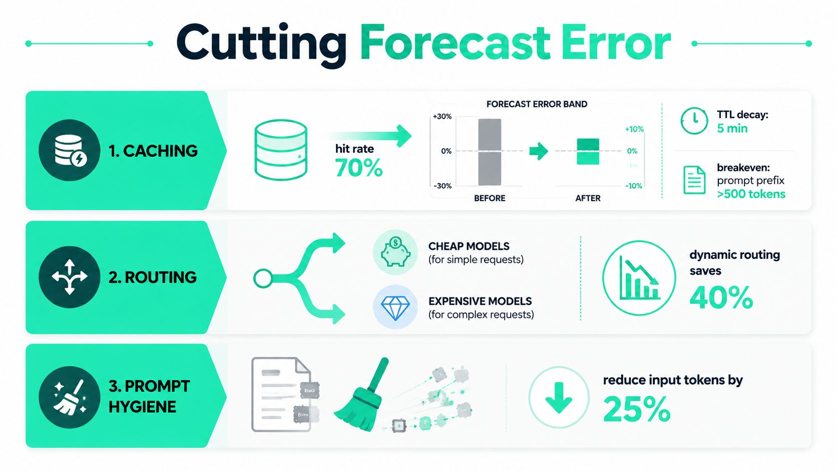
Three levers usually create the largest forecast changes: cache behavior, model routing, and prompt shape. Model each as a variable with an observed baseline, a plausible downside, and a test that can replace the assumption with telemetry.
Caching changes the input rate
Separate fresh input from cached input, then forecast the cache hit rate and its decay under real traffic. Repeated system prompts and stable context blocks can produce meaningful savings, but a cache strategy that works in a test environment may weaken when requests arrive outside the reuse window.
OpenAI prompt caching bills cached tokens at 50% off and applies automatically when prompts exceed 1,024 tokens and are reused within about 5 to 10 minutes, according to this guide to reducing AI token costs. Providers differ, so store the price-sheet version and cache rules with every forecast. Test the breakeven point against prefix size, cache writes, TTL decay, and the actual repetition pattern.
Routing trades quality against unit cost
Route routine extraction, classification, and short transformations to a smaller model when evaluation results support it. Keep complex reasoning, sensitive workflows, and failure-prone tasks on the more capable tier.
A useful routing forecast doesn't claim that every diverted request saves the same amount. It records the traffic share, expected token profile, model price, quality threshold, and rollback condition. The cost-management analysis covering caching, routing, and compression reports possible savings ranges of 50% to 90% from prompt caching, 40% to 85% from model routing, and 20% to 40% from prompt compression, with combined optimization sometimes reaching 60% to 90%. Treat these as scenario ranges from that source, not guaranteed outcomes.
Prompt hygiene reduces the numerator
Remove duplicated system instructions, trim stale few-shot examples, compress retrieved passages, and constrain unnecessary output. A neutral industry guide reports that prompt compression, context management, and output constraints can reduce input token costs by 20% to 40% in many use cases, while restructuring system prompts can cut prompt length by 30% to 50% in many cases without quality impact, as described in this LLM spend optimization guide.
Use probability-weighted scenarios instead of one fixed saving:
- Baseline: Current hit rate, routing mix, prompt length, and output distribution.
- Expected case: Tested cache reuse, approved routing rules, and measured prompt reduction.
- Stress case: Cache misses, fallback activation, longer responses, and traffic concentration.
Token-budget-aware reasoning can also lower output consumption. The TALE method reduced output tokens by 62.6% on Yi-lightning, 61.5% on GPT-4o-mini, and 69.8% on GPT-4o versus Vanilla CoT, with the reported GPT-4o-mini cost moving from 81.56 to 45.60 and GPT-4o from 1359.42 to 759.95, according to the TALE research paper. Validate quality before adopting the technique in production.
Validating Forecasts and Running Cost Incidents
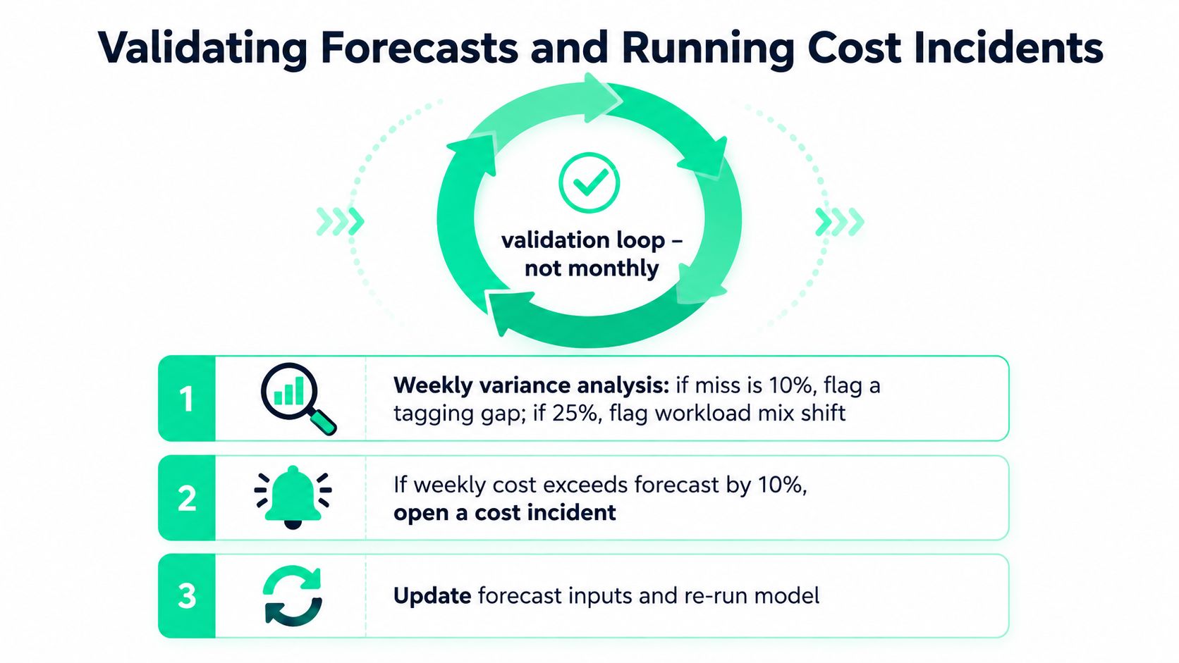
A forecast becomes useful only when the team compares it with actual usage often enough to catch drift. Monthly review is too slow for a feature that can change its prompt, routing, or traffic pattern in one deployment.
Run a continuous validation loop
Review variance weekly by provider, model, workflow, tenant tier, and product surface. Use thresholds to decide what happens next:
- 10% miss: Flag a tagging gap or telemetry mismatch.
- 25% miss: Investigate workload-mix changes, prompt expansion, or fallback frequency.
- 50% miss: Open a cost incident and assign an on-call owner.
These thresholds are operating rules for a runbook, not universal industry standards. Teams should tune them to their budget and traffic volatility, but they must define an escalation path before the invoice arrives.
Use named triggers during an incident
A cost spike becomes easier to handle when the alert names a likely cause. Build the runbook around triggers such as:
- Traffic surge: Check rate limits, request volume, tenant concentration, and recent launches. Confirm whether legitimate demand or an abusive client is driving the increase.
- Cache miss cliff: Compare fresh input against cached reads, inspect TTL behavior, and verify that prompt prefixes remain stable. If cache efficiency dropped after a template change, roll back the prompt or restore the reusable prefix.
- Rogue feature flag: Identify the feature, tenant, or environment that changed model routing. Roll back the flag, downroute eligible traffic, and preserve a sample of affected requests for analysis.
- Model fallback: Check provider errors, retry loops, and fallback frequency. A fallback model can alter both input and output economics without changing the product surface.
Use AI cost anomaly detection practices to connect alerts to ownership and remediation rather than merely notifying a finance channel.
The post-mortem should record the root cause, affected owner, customer impact, duration, triggering deployment, and corrective forecast adjustment. Feed the actual cache rate, output distribution, retry rate, and workload mix back into the input registry. The next forecast should inherit observed behavior, not preserve assumptions that the incident disproved.
A 30/60/90 Plan for Honest AI Cost Estimation
The rollout works best when engineering, finance, and product share artifacts rather than passing a spreadsheet between meetings. Assign one owner for each phase, define one checkpoint, and keep the evidence in the same system used for deployment and review.
Days 1 through 30
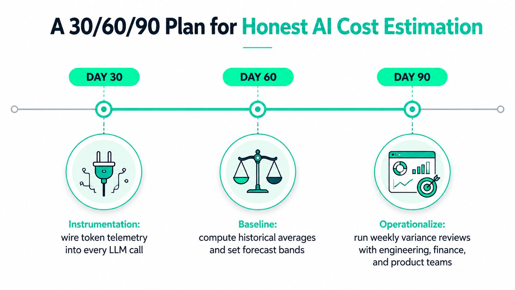
The first phase is instrumentation. Wire token telemetry into every LLM call, tag requests by feature and tenant, record model versions, and ship a dashboard that reconciles internal events against the vendor invoice to within 5%.
- Owner: Platform engineering.
- Checkpoint: Every production call has request-level usage and allocation metadata.
- Proof: A reconciliation dashboard and a documented event schema.
Don't start with optimization. If the data is incomplete, a cheaper model recommendation may just move unmeasured spend somewhere else.
Days 31 through 60
Build workload-segmented models for each major use case. Give chat, retrieval, summarization, embeddings, and agent workflows separate assumptions for volume, input, output, cache behavior, and model mix. Run weekly forecast-versus-actual reviews and publish a variance report that names the segments that drifted and why.
- Owner: FinOps or an engineering manager.
- Checkpoint: Every material workload has baseline, expected, and stress scenarios.
- Proof: A versioned forecast with variance commentary and approved assumptions.
SpendLens AI can serve as one implementation option. Its developer instrumentation and dashboard are designed to attribute OpenAI and Anthropic usage by project, provider, model, and workload, while surfacing cache efficiency, prompt waste signals, and model-switch opportunities. Teams can also use warehouse queries, provider exports, or an internal observability pipeline if those tools already provide the required detail.
Days 61 through 90
Operationalize the practice. Add anomaly alerts for per-segment spend velocity, connect the cost-incident runbook to on-call ownership, and recalibrate unit economics whenever provider pricing or model behavior changes. Quarterly recalibration is a minimum planning rhythm, not a substitute for weekly variance checks.
- Owner: Product and engineering leadership together.
- Checkpoint: Cost review becomes part of release and planning cadence.
- Proof: Incident history, updated forecast inputs, and a signed review record.
A forecast that survives this process does more than predict a bill. It shows which customers and features create value, which prompts waste tokens, where routing can reduce spend, and how much financial exposure a launch carries before the launch reaches production.
If your LLM bill still arrives as one unexplained provider total, start by instrumenting request-level tokens and workload metadata this week. Visit SpendLens AI to review a practical way to track OpenAI and Anthropic spend, identify cost drivers, and turn model-switch or prompt-optimization ideas into estimated monthly savings.