
How to Calculate Cost Savings from LLM Optimizations
Learn how to calculate cost savings from LLM optimizations with proven formulas, baselines, and risk checks. A practical guide for engineering and FinOps teams.
Your AI team has just shipped a prompt rewrite. Token usage falls sharply, the dashboard turns green, and the optimization gets added to the monthly finance update. Then the invoice arrives. The bill barely moved, or the apparent improvement disappears when traffic, model mix, and feature adoption are considered together.
That outcome is common because how to calculate cost savings involves more than subtracting one bill from another. A defensible LLM savings claim needs a comparable baseline, workload-level attribution, a clear record of the change that caused the difference, and a confidence assessment that shows how much of the result you can reasonably defend.
Table of Contents
- The Cost Savings Illusion Most LLM Teams Fall For
- The Core Formulas Behind Every Cost Savings Calculation
- Capturing Baseline Metrics and Attributing Savings to Specific Changes
- Gross Savings vs Net Savings and the Effective Savings Rate
- Estimating Confidence Risk and Migration Cost Before You Claim a Win
- Mapping the Workflow to SpendLens AI
- Building a Repeatable Savings Habit for LLM Spend
The Cost Savings Illusion Most LLM Teams Fall For
An AI team at a SaaS company rewrites a summarization prompt and celebrates a 40% drop in monthly token usage. The result looks decisive. Engineers point to shorter outputs, product accepts the change, and finance hears that inference efficiency has improved.
Two months later, the finance partner checks the actual spend. The number hasn't moved in the way the team expected. The team had compared traffic before a model release with traffic after a model release, while request volume was rising. The baseline also included a feature that had already been deprecated, so part of the token reduction came from workload removal rather than prompt optimization.
The team had measured an efficiency signal, not realized savings. Those aren't interchangeable.
Where the calculation broke
Several failure modes appeared at once:
- Mixed model versions: The old and new windows used different model pricing and behavior, so token counts weren't comparable without normalizing the rates.
- Traffic changes: A parallel increase in requests lifted the underlying cost, masking the savings from the prompt edit.
- Retired functionality: Deprecated traffic made the before-and-after comparison attribute unrelated savings to the prompt change.
- Blended reporting: Input and output tokens were combined, hiding which part of the workload changed.
- Missing ownership: No feature flag, release identifier, or experiment owner connected the savings claim to a specific production change.
A credible calculation needs four ingredients: a clean baseline, per-workload telemetry, attribution to a tagged change, and a confidence band. Without those, a percentage can describe what happened in a dashboard while saying little about what finance can book, forecast, or defend.
Practical rule: A token reduction is evidence of an optimization. It becomes a savings claim only after you show the comparable spend baseline and isolate the cause.
The basic cost-savings method remains useful. You subtract the new cost from the original cost, then divide the savings by the original cost and multiply by 100 for the percentage, as documented in this cost reduction calculator explanation. The hard work is deciding which costs belong in the comparison and how confidently you can attribute the difference.
The Core Formulas Behind Every Cost Savings Calculation
Keep four calculations on a reference card. Each answers a different finance question, and none replaces the others.
Absolute savings
Absolute savings = baseline cost − current cost
Suppose an LLM workload cost $42,000 per month before an optimization and $28,500 per month afterward. The absolute savings are $13,500 per month. This is the number finance needs for budget impact, but only if both figures cover the same workload, period, model basis, and traffic definition.
Percentage savings
Percentage savings = absolute savings ÷ baseline cost × 100
Using the same figures, $13,500 ÷ $42,000 × 100 = 32.14%, which can be reported as 32% when rounding is appropriate. A larger token reduction can still produce a smaller dollar reduction when the changed tokens represent a less expensive portion of the bill.
Annualized run-rate savings
Annualized savings = period savings × 12 ÷ period length in months
If the $13,500 monthly difference holds, the annualized run rate is $162,000. For a two-month pilot that produced $13,500 total savings, the annualized run rate would be $81,000, calculated as $13,500 × 12 ÷ 2. Label this clearly as a run rate, not realized annual cash savings. A pilot may not persist, and implementation costs may still be outstanding.
Per-unit economics
A workload-level total can hide volume changes. Track cost per 1,000 requests, cost per resolved ticket, or cost per generated document alongside total spend. For example, if a classification path moves from $3.10 to $0.74 per 1,000 requests, the unit difference is $2.36. At constant volume, multiply that difference by the number of 1,000-request units to estimate total savings.
The cost of API reference is useful when you need to keep provider pricing and token categories separate. Don't mix prompt tokens with completion tokens, and don't round input and output usage into one blended rate before calculating. The same logic applies to recurring expenses. A monthly reduction of $2,700 becomes $32,400 over 12 months, and the corresponding reduction is 21.6%, as shown in this recurring cost savings calculator example.
| Formula | Definition | Worked LLM Example | Result |
|---|---|---|---|
| Absolute savings | Baseline cost minus current cost | $42,000 − $28,500 | $13,500 monthly savings |
| Percentage savings | Absolute savings divided by baseline, multiplied by 100 | $13,500 ÷ $42,000 × 100 | 32.14% |
| Annualized run rate | Period savings multiplied by 12, divided by window length | $13,500 × 12 ÷ 2 | $81,000 annualized |
| Per-unit savings | Unit cost before minus unit cost after | $3.10 − $0.74 per 1,000 requests | $2.36 per 1,000 requests |
Capturing Baseline Metrics and Attributing Savings to Specific Changes
A savings calculation starts before the optimization ships. Capture spend at the level where a team can take action, such as model, environment, feature flag, endpoint, and workload. A company-wide invoice is useful for reconciliation, but it can't tell you whether a prompt edit, model switch, cache rollout, or traffic change produced the result.
Use a stable baseline window long enough to represent normal behavior, commonly 14 to 28 days, while recording request count, input tokens, output tokens, cache hits, and blended cost per request. The source for each observation should also include the production prompt version, deployment identifier, model version, and any feature flags active during the window.
Tie each result to one change
A model switch is easiest to attribute when the workload stays constant. A classification workload that falls from $3.10 to $0.74 per 1,000 requests has a unit-cost difference of $2.36, but the claim is only defensible if the request definition and classification quality remain comparable.
Prompt edits require a different view. If average output tokens fall from 412 to 238 on a summarization feature, record the prompt revision and compare output-token cost separately from input-token cost. Shorter output may reduce spend, but it can also affect summary completeness, retries, or downstream processing.
Caching needs its own metric. If a retrieval path's cache-hit rate rises from 12% to 61%, report the change alongside request volume, cacheable-token volume, latency, and provider billing behavior. A higher hit rate isn't automatically equivalent to a particular dollar amount unless the provider's cache pricing and returned usage fields support that calculation.
Savings should trace to one tagged change, one owner, and one before-and-after window.
A practical schema might include workload, owner, purpose, model, environment, release, input_tokens, output_tokens, cache_hits, requests, and cost. The best practices for reporting LLM spend can help teams turn those fields into a report finance can audit without reconstructing the analysis from application logs.
Don't aggregate unrelated changes into one launch result. If a prompt edit and model switch shipped together, call the outcome a combined optimization unless a controlled comparison separates their effects.
Gross Savings vs Net Savings and the Effective Savings Rate
A 35% token reduction rarely produces a matching 35% cost reduction. Token categories can carry different prices, some tokens may not be billable in the same way, and request growth can consume the benefit. Engineering work, migration windows, parallel inference, testing, and observability also reduce what the business keeps.
Start with gross savings, then reconcile the costs required to achieve it:
Net savings = gross savings − implementation cost − migration cost − parallel-run cost
Consider a quarterly LLM migration with $48,000 gross savings. Engineering time costs $12,000, and running both inference paths during cutover costs $10,000. Net savings are $26,000.
| Line Item | Quarterly Amount | Notes | Cumulative Net Savings |
|---|---|---|---|
| Gross savings | $48,000 | Reduction against the approved baseline | $48,000 |
| Engineering implementation | −$12,000 | Instrumentation, testing, and rollout work | $36,000 |
| Parallel inference | −$10,000 | Temporary duplicate serving during cutover | $26,000 |
Migration cost may also include downtime, training, validation, rollback preparation, and changes to dependent services. An independent cost savings guide makes the same important distinction: gross savings alone can overstate year-one ROI when setup and adoption costs are material.
Choose the right savings rate
The Effective Savings Rate, or ESR, is strongest when it uses On-Demand Equivalent spend rather than raw invoice reduction. The FinOps savings calculation guidance defines ESR as savings generated divided by ODE spend, and relates it to commitment utilization, coverage, and discount. For LLM workloads, adapt the principle by defining the pre-optimization spend basis clearly, then report both gross and net rates.
Using the worked figures above, the net savings rate against a $100,000 quarterly pre-optimization spend would be 26%, while gross savings would be 48%. Those percentages describe different realities. The first reflects what remains after implementation and cutover costs.
Before publishing a result, ask:
- Vanity metric: Is the claim based only on tokens, cache hits, or model calls?
- Temporary cost: Have parallel-run and migration charges been removed?
- Stable baseline: Has the post-migration workload settled enough to replace the temporary comparison?
- Audit path: Can each dollar trace back to workload-level measurements?
Retire the original claim once the post-migration baseline stabilizes. Replace it with the realized run rate and the costs required to maintain it.
Estimating Confidence Risk and Migration Cost Before You Claim a Win
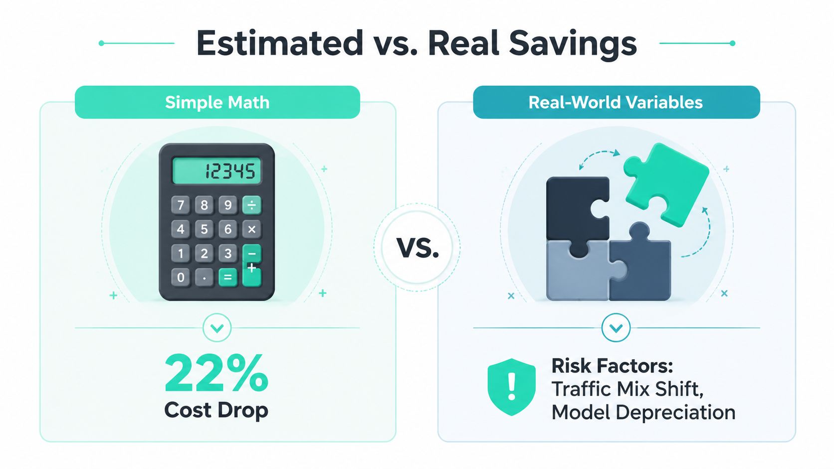
A percentage cut can be real in the observed window and still fail as a forecast. A 22% reduction traced to one prompt edit may disappear when traffic mix changes, a model is deprecated, or users shift toward longer requests. The number isn't useless. It needs a confidence label.
Use three practical bands:
- Low confidence: One observation with no holdout or controlled comparison.
- Medium confidence: Two weeks of post-change data across a mixed workload.
- High confidence: Four weeks of controlled data with traffic held constant.
These bands describe evidence quality, not business value. A small, high-confidence win may deserve priority over a larger, low-confidence result.
Price the risk before rollout
Score migration risk using the factors your team can observe:
- Engineering effort: How much implementation and validation work does the change require?
- Rollback complexity: Can the previous model or prompt return immediately?
- Dependency surface: How many services, user flows, and downstream systems depend on the output?
Record the score beside the savings estimate. A model replacement with simple rollback and limited dependencies should not receive the same treatment as a provider change embedded in customer-facing workflows.
You can convert evidence quality into a risk-adjusted estimate:
Risk-adjusted savings = gross savings × confidence multiplier − migration cost
Use a 0.5 multiplier for a low-confidence result, 0.75 for medium confidence, and 0.9 for high confidence. If gross savings are $20,000 and migration cost is $4,000, the estimates are $6,000, $11,000, and $14,000 respectively after applying those multipliers and subtracting the migration cost.
A low-confidence saving belongs in the experiment ledger, not in the committed finance forecast.
The AI observability platform overview is relevant when teams need the workload, release, token, and cost signals required to support this review. Publish a win only when the baseline is comparable, the change is tagged, quality is checked, and the migration score has an owner.
Mapping the Workflow to SpendLens AI
The calculation becomes repeatable when instrumentation follows the same path as the financial question. Start with Per-Workload Spend reports. Break costs down by project, provider, model, environment, and feature, then compare token counts, cache efficiency, request volume, and per-call cost within a consistent workload definition.
Next, use Change Tracking to connect the difference to a model switch, prompt revision, cache rollout, or release. A change log should preserve the before-and-after windows, owner, feature flag, and deployment context. This prevents a later review from treating a traffic shift as an optimization.
Wire the signals in sequence
SpendLens AI can map the operating workflow as follows:
- Tag workloads: Use workload, task, feature, experiment, or endpoint tags so each call has an accountable owner and business purpose.
- Enable change logs: Record model changes, prompt versions, cache rollouts, and deployment dates beside the spend data.
- Run the Savings Calculator weekly: Ingest baseline and current cost to produce absolute, percentage, and annualized views, while keeping unit economics visible.
- Export risk-adjusted results: Require confidence and migration-risk fields before a number enters a finance report.
The calculator should surface ESR as a separate measure, not hide it inside a headline percentage. Alerting thresholds should monitor cutover spend, parallel inference, unusual token growth, and unexpected changes in cache efficiency. An alert that arrives during migration is more useful than a post-invoice explanation.
A sample SpendLens AI report shows the kind of executive-ready output teams can use to connect spend drivers with recommendations. The useful design principle is separation. Engineers need per-call and per-workload evidence, while finance needs a concise reconciliation that explains gross savings, costs, confidence, and realized run rate.

Don't start with every dashboard feature. Start with tags, change history, baseline snapshots, and a review export. Those four signals support the calculation before the organization invests in more elaborate reporting.
Building a Repeatable Savings Habit for LLM Spend
LLM optimization works better as an operating rhythm than as a one-time cost project. The team should be able to explain what changed, what it saved, what it cost to implement, and how confident it is that the result will persist.
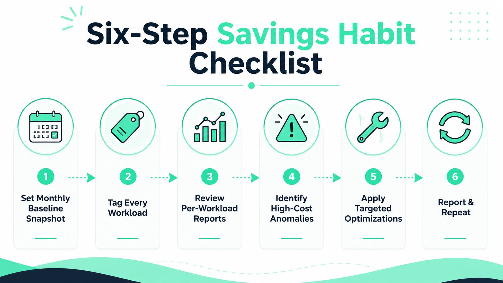
Use this six-step rollout checklist:
- Set a monthly baseline snapshot: Preserve spend, request volume, token categories, cache behavior, and active model versions.
- Tag every workload: Assign an owner, purpose, product area, environment, and feature identifier.
- Review per-workload reports: Compare like-for-like operations rather than relying on a provider-wide invoice.
- Identify high-cost anomalies: Investigate unusual prompts, output growth, model mismatches, and cache deterioration.
- Apply targeted optimizations: Test model right-sizing, prompt edits, caching, batching, or routing with a recorded counterfactual.
- Report and repeat: Publish realized savings, implementation costs, confidence, and the next review date.
Three habits make the system compound. Run a quarterly prompt audit to find oversized templates, repeated instructions, unnecessary context, and long outputs. Review cache-hit rate alongside latency budgets, because aggressive caching may change freshness or response behavior. Schedule a model right-sizing day for small, well-bounded workloads, then test cheaper candidates against quality and reliability requirements.
Keep a counterfactual for every meaningful change. If the model switch hadn't happened, what would comparable workload spend have been? That answer gives finance a baseline for savings, while the implementation ledger captures the cost of creating the difference.
Teams that run this cycle for four consecutive quarters can move from ad-hoc token cuts to a predictable, audit-ready program, but the process still matters more than the calendar. Re-baseline after model pricing changes, retire stale claims, and separate realized savings from opportunities that haven't survived production.
SpendLens AI provides workload-level LLM spend tracking, change attribution, savings calculations, confidence and migration-risk signals, and reporting for OpenAI and Anthropic workloads. Visit SpendLens AI to tag your workloads, test optimization opportunities, and produce a risk-adjusted savings view finance can review.